- Home
- »
- FAQ
Frequently Asked Questions
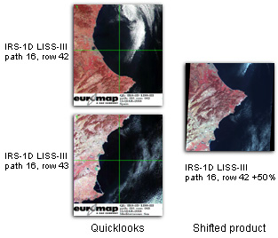
Can Scenes be shifted?
For the appropriate coverage of an area of interest all IRS data products, except IRS-P6 LISS-III quarter scenes, can be shifted southwards along the satellite track. A shift along track can be chosen in increments of 10 % with regard to the respective scene size. This means a 10 % shift along track corresponds to 14 km for a 140 km x 140 km LISS-III full scene but to 7 km for a 70 km x 70 km LISS-III quarter scene.
It is not possible to shift scenes in an East-West direction across the track.
What is the Field of View (FOV) and where can I find it?
In general, the Field Of View (FOV) describes the opening angle of a camera’s optic. The opening angle and the camera’s altitude above the ground (distance between camera and object) determine the size of the imaged area (swath width).
For IRS cameras, the cross track FOV can be found in the Super Structure Format or on the pages describing the IRS-1C, IRS-1D and IRS-P6 cameras. The cross track Field Of View in radiant for one pixel is given.
p = tan(FOV) * a
s = n * tan(FOV) * a
where: a – camera’s altitude above ground (m)
FOV – cross track Field Of View
p – size of a pixel cross track (m)
s – swath width (m)
E.g. for IRS-1C LISS-III this is:
p = tan(0.0000288) * 817000 m
p = 23.5 m
s = 6000 * tan(0.0000288) * 817000 m
s = 141177 m
s = 141 km
What has to be observed while performing an ortho correction using RPCs from IRS-P6 Ortho-Kits?
As pointed out in the ResourceSat-1 Geometric Accuracy Assessment, IRS-P6 RPCs should be used with image-space polynomial correction terms. A first-order polynomial correction is sufficient for LISS-IV, LISS-III and AWiFS B and D scenes. For AWiFS A and C scenes, a second-order polynomial correction is required.
For GAF’s test results see the following slides.
How are Radiances calculated?
The values given for GAIN and BIAS in the header are not the GAIN and BIAS as expected. These values are L_min and L_max, given in units of mW/(cm*cm)/str/micron, where BIAS is L_min and GAIN is L_max.
D
L_rad = ——- * ( L_max – L_min ) + L_min
G_max
where:
L_rad is the radiance
G_max = (2 ^ Q) – 1
Exception: G_max = 255 for IRS-1C and IRS-1D radiometrically corrected and higher level products.
L_max is the maximum saturation radiance
L_min is the minimum saturation radiance
D is the DN from the image
Q is the number of quantisation bits of the sensor
.
What are the at-sensor solar exoatmospheric irradiances of the IRS cameras?
The at-sensor solar exoatmospheric irradiance and Rayleigh optical thickness can be found at the end of the NRSC reports for IRS-1C/1D/P6 and Resourcesat-2.
Can I load IRS-1D data in IMAGINE?
Yes, you can.
IMAGINE 8.4
contains an importer for IRS-1D data
IMAGINE 8.3
IRS-1D data can be imported by using the IRS-1C importer (IRS-1C Euromap Fast Format C). The import procedure is slightly different, because we had to expand the naming conventions for IRS-1D. Therefore the IRS-1C importer is unable to identify the data and header files automatically.
You will find an import example for IRS-1D PAN and LISS data sets below.
PAN data
- choose Import | Euromap IRS-1C (Euromap Fast Format C)
- Media: File
- select Input-Directory + File: e.g. f:/24_34D/H0D0Y867.07A (header file according to the naming conventions [the smaller of the two files])
- enter Output-Directory + File: <output>
- now click OK
- in the “IRS-1C Band File Error” dialog-box that appears, click Select Band File(s)
- select the data file (e.g. H0D0Y867.070) in the window that appears
- assign this file to band 1 by using the button Band # 1 SET
- now click OK and the “IRS-1C Information” should display all header information correctly
- from here you can proceed as usual: i.e. click Preview or OK to read the entire scene
LISS data
- choose Import | Euromap IRS-1C (Euromap Fast Format C)
- Media: File
- select Input-Directory + File: e.g. f:/24_34Q4/N0O0Y867.0FL (header file according to the naming conventions [the smallest file])
- enter Output-Directory + File: <output>
- now click OK
- in the “IRS-1C Band File Error” dialog-box that appears, click Select Band File(s)
- in the window that appears select the data files which correspond to data channels
e.g. N0O0Y867.0FM = band 1
and N0O0Y867.0FN = band 2 … etc. - assign the file N0O0Y867.0FM to band 1 using the button “Band # 1 SET”,
assign the file N0O0Y867.0FN to band 2 using the button “Band # 2 SET” … etc.
until all four bands are selected. The optional synthetic blue channel has to be read instead of one of the four LISS bands or has to be imported later as a separate band. (five bands can not be imported as “LISS” at the same time) - now click OK and the “IRS-1C Information” should display all header information correctly
- from here you can proceed as usual: i.e. click Preview or OK to read the entire scene
(Translated from the German version of an old Geosystems FAQ.)
How can I load IRS PAN products in Super Structure Format in IMAGINE?
IMAGINE 8.5 and 8.6 contain Super Structure import modules. Unfortunately, the import module expects the Super Structure files to follow a naming convention of unknown origin. The official Super Structure format document does not define any naming conventions at all.
The names accepted by IMAGINE are as follows:
Volume.pan
Leader.pan
Imagery.pan
Trailer.pan
Null.pan
In order to use the importer for IRS PAN products rename the Super Structure files as listed above. E.g. rename IRS PAN Super Structure products from GAF as follows:
a00.vol -> Volume.pan
b00.led -> Leader.pan
c00.img -> Imagery.pan
d00.trl -> Trailer.pan
e00.nul -> Null.pan
Leica Geosystems and GAF are working on a solution. A patch Fix19209.860.EXE exists but was not released due to limited resources. Leica Geosystems will probably incorporate the solution in release 8.7.
Can I view images stored in the Fast Format with Adobe Photoshop?
Yes, you can view images stored in the Fast Format with Adobe Photoshop. What you cannot do with Photoshop is use the geometric information included with the product.
For panchromatic data you simply have to load the image file, that’s all.
In the case of multispectral data, you must load the data band by band. That way you can see each separate band. If you have loaded three or more channels, you can merge these channels to create an RGB image (look for Merging channels in the online help). If you have less then three bands, you have to duplicate one of the bands (look for Duplicating channels in the online help) before you can create an RGB image by merging the channels.
To load one image file (one channel of the product) do the following:
- Select Open As from the File menu.
2. Select Raw (*.RAW) as the format from the Open As list box. Now select an image file to load.
Check that you really have selected an image file by looking at the bottom line of the dialog where the size of the selected file is displayed. The size of header files is around 5 Kbytes and the size of image files is in the range of Mbytes.
3. A dialog where you can specify how the image should be loaded is displayed. Photoshop fills in values which describe the image correctly in more than 95% of cases, so that you can simply press the OK button to see what happens.
If you are confronted with more dialog boxes, or you only see garbage instead of an image, you have to start with step 1 again. You have to fill in the correct values for the Width and Height of the image in the dialog. These values can be found in the header file included with the Fast Format product:
PIXELS PER LINE = 2987
LINES PER BAND = 2880
The other values are always as displayed.
